(All code used in this ‘benchmark’ can be found in this gist.)
Almost 2 years ago, I installed Julia for the first time and tried to implement some algorithms that I use in my research (mainly Bayesian models). At that time, I fairly quickly got frustrated because of uninformative error messages, and the lack of documentation (whether official or forums) to help me out.
Now that version 0.4.0 got out, I decided to give it another try. Having to write MCMC algorithms all the time, speed is an important issue. My normal workflow is to develop new models in R and once I have a working prototype, I translate the (slow) MCMC core of the method in Fortran (not FORTRAN) for speed and call the Fortran routines from R. Why I prefer Fortran over C/C++ cannot be better explained than in this blogpost.
Julia promises a performance that is close to these lower level, compiled languages as Fortran and C++, but with the advantage of a REPL. Sounds promising enough to give it a second try.
The model I choose for this investigation is the Bayesian binary probit model:

with:
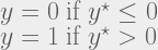
The typical Bayesian approach for this model is to treat the latent variable y* as any other unknown parameter. Then, conditional on (the simulated) y*, the problem reduces to the well-known linear regression model. An efficient Gibbs sampler for this model was first discribed in Albert & Chib (1993).
This model is well suited for comparing the performance of R, Julia and Fortran, because of the loops within loops that are required by the Gibbs sampler. That is, in each MCMC iteration, a latent y* has to be simulated from the truncated normal distribution for each observation. It is well-know that this type of algorithm is very slow in interpreted languages as R (or Python).
For this benchmark, 5000 observations were simulated from the probit model, each containing two covariates plus an intercept. The dependent variable is binary. This data was then stored as a csv file that was then read by the different software implementations. The MCMC algorithm in each implementation was run for 5000 iterations (leading to 25 million calls of Geweke’s accept-reject algorithm (1991) for the truncated normal draws). The calculated execution times only relate to the execution of the MCMC algorithm (not reading in data, etc.).
The runtimes presented below is the average over 5 executions of the code on the same dataset. I ran the code on my (very) old Dell Vostro 1000 laptop (CPU: AMD Turion 64 X2 TK-57, MEM: 3 Gb DDR2, OS: ArchLinux). R version 3.2.2, Julia version 0.4.0 and the Fortran compiler I used was gfortran (GCC 5.2.0) with the -03 optimization flag. Note that the Fortran code should be compiled against the LAPACK library.
The results are given below:

As expected, Julia outperforms R by a large margin (almost 25x faster). However, Fortran is still about 4x faster than Julia in this specific exercise. Note that I did not follow the strict rules that real benchmark studies require, so these results are only indicative of the real performance differences between the programming languages for this problem.
What I learned from this exercise is that Julia really has matured a lot in the last 2 years. Error messages are more informative what makes debugging easier. And one can pick up the Julia syntax quite easily. Writing Julia or R requires more or less the same effort. Fortran is the clear winner here, but this however comes at the cost of slower and more painful development time.
I see myself using Julia much more often in the (near) future. For most of my work, it would take away the need to translate my prototypes in Fortran, and this would save quite some time. However, whenever speed is really crucial, Fortran is still the best option.
All code that was used in this benchmark can be found on this gist.
Final note: As I’m new to Julia, it’s possible that the code that I wrote is suboptimal, please comment if you find such inefficiencies. For the R code, I tried to vectorize as much as possible, thus writing the code as efficient as possible. In the Fortran code, I use the very efficient Cholesky facotrization to invert the variance covariance matrix, while I use the more general matrix inversion functions in R and Julia. However, since matrix inversions only appear outside the loops, this should not affect total runtime substantially.
